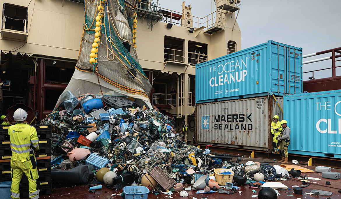
Tue Feb 27 2018

Who will win the football league? A data-driven prediction

This blog was written in 2018 with a focus on the Dutch football league. It had been updated in 2022 in light of the ongoing World Cup Championship. The prediction techniques remain relevant today even if the data they're using about the league is outdated.


The Dutch football league, de Eredivisie, is coming into the final stages. Nothing is decided yet, as the prizes will (usually) not be given out until May. The football matches played until now indicate which teams are the contenders for the title and which have to fear for relegation. In this blog, we will give a data-driven prediction of the winning football team.

Using multilevel modeling, we discovered a pattern in the football matches played until now. This pattern can be used to simulate the remaining matches. Using these simulations, we can predict an expected ranking. Our approach to learning this model is the Bayesian one, we will sample possible models using the python package pymc3.

The model

Football isn’t a complicated game. Two teams try to score by playing the ball into the other team’s goal. We model the number of goals for both teams as independent random variables. The parameters, which encode attacking potential, defensive capabilities and home advantages of each team, are learned from the football matches played.

This model is a variation on existing approaches. The hierarchical modelling of the home advantages may be new, but we haven’t seen it before. The model is pretty simple and doesn’t take into account current form or the fact that Robin van Persie just joined Feyenoord.

Results

Before diving into the implementation details, we provide an overview of the results. This is to accommodate all you coaches on the couch who are not necessarily interested in non-centered specification! Let’s first look at the parameters that the model has inferred for the Dutch teams. We sorted the positions on attacking rate.

The attack rate corresponds to the number of goals scored on average, while the defense rate is a score that measures the number of goals prevented. In fact, on average, ignoring the home advantage, this model estimates the number of goals in the next football match between Vitesse and AFC Ajax for example.

This is a tight matchup. Which might swing in favor of AFC Ajax. At the moment, PSV is leading the competition. Our model thinks AFC Ajax does slightly better on both offence and defense. This is not surprising considering that Ajax has scored more and accepted less goals this year. Feyenoord, fifth in the ranking, does not have the scoring potential to challenge the first two. However, they are defending among the best.

Most teams in the Dutch competition seem to lower their defenses at home while increasing their scoring potential, perhaps to offer their home crowd a good show? Only PSV, AFC Ajax, PEC Zwolle, and Heracles Almelo defend better at home.

If we run simulations based on these ratings, the results at the end of this season are predicted as shown below. The table below represents the probablity that each club ends up in each of the given ranks.

According to this model, PSV is the big favorite. They have a seven-point lead over AFC Ajax at the moment. However, with their good scoring potential and solid defense, the model gives AFC Ajax a 15% probability of winning the competition.

Positions are less certain at the bottom and the middle of the pack, where a single victory can make a large difference in terms of ranking. The model predicts a lower final ranking for PEC Zwolle, ranked 6th at the moment. This is a reasonable prediction if you take into account their current goal tally.

The same model is applied to the big leagues in Europe. You can find the results of these models below. It’s interesting to note that the Dutch league is one of the more exciting competitions. The victories of super teams like FC Bayern München, FC Barcelona, and Manchester City seem certain. The most exciting competition is the Italian Serie A, with Juventus being the only slightly more likely to win the competition than SSC Napoli.

Model evaluation

What this approach does not accommodate for, is the effect of a new trainer appointed during the winter break. No ‘Dick Advocaat –‘ (Sparta Rotterdam) or ‘Erik ten Hag –‘ (AFC Ajax)  effect can be predicted. The effect of a transfer is also not estimated directly. Basically, the model infers the strengths over the season so  far and extrapolates this over the rest of the season. As such, it is probably too certain of the outcome, as transfer effects, injuries, and changes in form can really make the second half of the season different from what we have seen so far.

The first thing to incorporate in this model would be something that tracks the changes in form over the season. Additionally other effects as for example the weather, referee or time of day that a football match is played. There is also a real effect of fatigue, some teams play multiple football matches in a week because they’re involved in a European League or the National Cup. The effect of fatigue will matter less in the second half of the season. Dutch teams traditionally don’t reach the second round in these competitions. However, it could influence the interpretation of earlier results. It would be interesting to be able to check how big this effect is. The cool thing about this model in pymc3 is that it is relatively easy to expand the model and add extra parameters if you, as a data scientist and part-time  football coach, think it is of importance.

A necessary step that we omitted here is an evaluation of this model over the previous years.

That said, these simulations lead to what we think are very reasonable probabilities. Taking well into account the strength of the opponents played and those that are still on schedule. The model might also be useful in practice to give teams an indication of what they should improve on.

It is nice that we needed a relatively small amount of data in order to learn this model. In the age of Big Data, not all data sets are large and this technique offers a great way to build robust models. That also  gives some certainty about their uncertainty. Additionally, it is possible to interpret the parameters in the model. This all makes  Bayesian multilevel modelling extremely powerful. Thanks also to the NUTS-sampler of course, and the pymc3 developers that makes it so accessible.

As a bonus, we give predictions for the big leagues down here. After that, it will be Nerds Only, as we dive into the implementation. If  you’re interested in more details, or up-to-date predictions, feel free to reach out!

Als ik zou willen dat je het begreep, dan had ik wel beter uitgelegd!
Johan Cruyff

Bundesliga

In Germany, their best team is FC Bayern München. Given their current point advantage, we’re very sure they will win. After the first position, things are still exciting with many teams in contention for second place. Funny note, compared to the Dutch league, the home advantages are much larger in Germany.

Bundesliga predictions

Bundesliga estimated team stats

Bundesliga football team stats

Primera Division

In Spain, the top spot is pretty much taken. Atlético Madrid is also pretty certain of its second place. This is not due to their scoring potential, but their defensive capabilities have shown to be rivalled only by FC Barcelona (the number 1).

Primera Division predictions: The possibility for each team ending end up at each rank

Primera Division estimated team stats

Primera football team stats

Series A

This is the most exciting competition. Both Juventus and SSC Napoli are in real contention for the overall win. Teams are not especially defensive when playing at home and the home advantages are not as large as in the German division.

Serie A predictions

Serie A football predictions

Series A estimated team stats

Serie A football team stats

Premier League

In England, we are confident about Manchester City ending up on the top spot. Again, there are some interesting differences in defensive capabilities. Burnley FC is doing well, despite having a very low goal count. West Bromwich Albion FC, the current lowest ranked team, still have chances of reaching up to 15th or even 12th position.

Premier League rank predictions for each team

Premier League estimated team stats

Premier League football team stats

Implementation

We implement a Bayesian multilevel model using,pymc3 a  package that implements the No-U-Turn-Sampler and is built on Theano. To understand what’s going on requires knowledge of Bayesian modelling and  the pymc3 package. If you’re new to that, we recommend for example the online workbook Probabilistic Programming and Bayesian Methods for Hackers.

We view a football match as two independent Poisson processes. Each produces a number of goals for each side. Using an exponential link function, the rate parameters are a sum of attacking rate, respective defense rates, and a bonus on both attacking and defending for the home team.

home goals ~ Poisson(exp(μhome))
away goals ~ Poisson(exp(μaway))

Where μ is the rate parameter in each direction.

# Import the necessary packages 
import pymc3 as pm 
import pandas as pd 
import seaborn as sns 

%pylab inline 
np.random.seed(10)

Populating the interactive namespace from numpy and matplotlib

# read in the data, downloaded from http://www.football-data.co.uk/data.php
comp = pd.read_feather("./data/nl_comp_07-02-2018.feather")
comp.sample(10)

The data is read from the feather format, and cleaning up has been done to make sure the data types are correct. In particular, we make use of the category type in pandas. In this post we use it a lot to translate between index positions in the pymc3 model and the team names.

For our "predictors" we use a theano.shared variable. The predictors contain 'which team was playing at home' and 'which team was playing away' for each football match. This allows us to change these predictors for the football matches that we want predictions for, and use the compiled model to efficiently sample simulations.

import theano

n_teams = len(comp.hometeam.cat.categories)
played = comp[comp.played]
not_played = comp[~comp.played] 

## create shared predictors
hometeam = theano.shared(played.hometeam.cat.codes.astype('int8').values)
awayteam = theano.shared(played.awayteam.cat.codes.astype('int8').values)

A good attack starts with a strong defense

In the first set of definitions below, we see the attack_rate for each team. This corresponds to the number of goals that each team scored in the first half of the season.

However, there is another important aspect to football, defense. In order to win games, a team must not only score goals, it also has to prevent the other team from scoring more than they do. And just as with scoring goals, some teams are better at this.

The first part of the model is the attack and defense rates for each team. These are vectors of length n_teams, and we put a hierarchical prior on these parameters, with weak hyperpriors. Keep in mind these parameters will be translated from log scale by the exponential link function. In this model, a non-centered version is necessary for efficient sampling. You can read the following blog for some background. Important point of note, make sure that the defense rates are centered on zero.

with pm.Model() as model: 
    attack_hyper = pm.Normal('attack_hyper', 0, 1) 
    attack_hyper_sd = pm.Gamma('attack_hyper_sd', 2, 2)
    attack_rate_nc = pm.Normal('attack_rate_nc', 0, 1, shape = n_teams)
    attack_rate = pm.Deterministic(
        'attack_rate', 
        attack_hyper + attack_rate_nc * attack_hyper_sd
    ) 
    defense_rate_nc = pm.Normal('defense_rate_nc', 0, 1, shape = n_teams)
    defense_hyper_sd = pm.Gamma('defense_hyper_sd', 2, 2)
    defense_rate = pm.Deterministic(
        'defense_rate', 
        defense_rate_nc * defense_hyper_sd
    )

The twelfth man

Another established effect on the outcome of a football is the home advantage. 60% of football matches are decided in favor of the home side. We determined that a team has both defensive and attacking qualities. We hypothesize that the home advantage can work on both these qualities. On these, we again use a hierarchical prior, with weak hyperpriors.

with model: 
    home_attack_hyper_sd = pm.Gamma('hahsd', 2, 2) 
    home_attack_hyper = pm.Normal('hah', 0, 1) 
    home_attack_nc = pm.Normal('hah_nc', 0, 1, shape = n_teams) 
    home_attack_advantage = pm.Deterministic(
        'home_aadv', 
        home_attack_hyper + home_attack_nc * home_attack_hyper_sd
    ) 
    home_defense_hyper = pm.Normal('hdh', 0, 1) 
    home_defense_hyper_sd = pm.Gamma("hdhsd", 2, 2) 
    home_defense_nc = pm.Normal('hdh_nc', 0, 1, shape = n_teams) 
    home_defense_advantage = pm.Deterministic(
        'home_dadv', 
        home_defense_hyper + home_defense_nc * home_defense_hyper_sd
    )

The number of expected goals for a team is the exponential of the sum of the right parameters.

with model:
    home_diff = (
        attack_rate[hometeam]
        - defense_rate[awayteam]
        + home_attack_advantage[hometeam]
    )
    away_diff = (
        attack_rate[awayteam]
        - defense_rate[hometeam]
        - home_defense_advantage[hometeam]
    )

The number of goals is a Poisson parameter with an exponential link. We're not accounting for any overdispersion, which is probably a weakness of the model. However, it won't influence the predictions that much.

with model: 
    home_goals = pm.Poisson(
        'home_goals', 
        pm.math.exp(home_diff), 
        observed = played.fthg.values
    ) 
    
    away_goals = pm.Poisson(
        'away_goals', 
        pm.math.exp(away_diff), 
        observed = played.ftag.values
    )

We use two chains to be able to assess the mixing. Sampling is quite efficient and takes half a minute on our laptop. The trace plot looks healthy!

with model: 
    trace = pm.sample(1000, tune=500, njobs=2) 
    pm.traceplot(trace);

With some data-fu, we reorganize the posterior samples to be able to compare the rates per team. To keep things readable, we only plot the medians, which will disappoint the true Bayesian warriors among you.

team_names = comp.hometeam.cat.categories 

post = pm.trace_to_dataframe(
    trace, 
    varnames=["attack_rate", "defense_rate", "home_aadv", "home_dadv"]
)
post = post.stack().reset_index() 
post.columns = "sample", "param", "value"
q = post.param.str.contains("__")
post.loc[q, "team"] = team_names[
    post[q].param.str.split("__").str.get(-1).astype(int)
]
post["type"] = post.param.str.split('__').str.get(0)

labels = { 
    "attack_rate": "Attack rate", 
    "defense_rate": "Defense rate", 
    "home_aadv": "Home attack advantage", 
    "home_dadv": "Home defense advantage"
}

ax = (
    post.groupby(["type", "team"])
    .value.median()
    .unstack(0)
    .sort_values("attack_rate")
    .rename(columns=labels)
    .plot.bar(subplots=True, figsize=(10, 10), legend=False)
)

plt.tight_layout()
Parameters

By setting new values for the shared predictor variables, we can use the compiled model to get some simulated outcomes. This is really quick, taking a couple of seconds for 1000 simulated competitions!

## simulate matches

hometeam.set_value(not_played.hometeam.cat.codes.astype('int8').values) awayteam.set_value(not_played.awayteam.cat.codes.astype('int8').values) 

with model:
    ppc = pm.sample_ppc(trace, samples = 1000)
    ppc 
100%|███████████████████████████████████████████████████████████████████████████████████████████████████████████████████████████████████████████████████████████████████████| 1000/1000 [00:00<00:00, 1540.72it/s] 

{
    'away_goals': 
        array([
            [2, 2, 0, ..., 2, 0, 1],
            [3, 1, 0, ..., 1, 0, 1],         
            [2, 0, 3, ..., 2, 1, 0],  
            ...,                
            [1, 1, 3, ..., 1, 2, 1],         
            [0, 1, 0, ..., 1, 0, 3],         
            [3, 2, 0, ..., 0, 2, 5]
        ]),  
    'home_goals': 
        array([
            [1, 1, 1, ..., 3, 0, 5],         
            [0, 0, 1, ..., 0, 2, 3],         
            [1, 4, 1, ..., 0, 0, 3],         
            ...,         
            [2, 2, 1, ..., 0, 0, 1],         
            [1, 1, 0, ..., 3, 1, 5],         
            [2, 2, 1, ..., 6, 1, 3]
         ])
} 
ppc["home_goals"].shape 
(1000, 81)

Now we have a 1000 simulated competitions, which has 81 football matches to be played. Each of these 1000 simulations is the full remaining match schedule. Let's have a look at 2 simulated outcomes for the home matches of AFC Ajax.

comp.loc[~comp.played, "ftag"] = ppc["away_goals"][0] 
comp.loc[~comp.played, "fthg"] = ppc["home_goals"][0] 

comp[(comp.hometeam == "Ajax") & ~comp.played]
comp.loc[~comp.played, "ftag"] = ppc["away_goals"][1] 
comp.loc[~comp.played, "fthg"] = ppc["home_goals"][1] 

comp[(comp.hometeam == "Ajax") & ~comp.played]

There is considerable variance here, but overall the predictions for AFC Ajax's home games are pretty positive.

Below, we show the ranking as a result of one simulation.

def get_standing(comp, ppc, simulation):
    comp.loc[~comp.played, "ftag"] = ppc["away_goals"][simulation]
    comp.loc[~comp.played, "fthg"] = ppc["home_goals"][simulation] 
    
    comp["homepoints"] = (
        3 * (comp.fthg > comp.ftag)
    ).fillna(0) + (
        1 * (comp.fthg == comp.ftag)
    ).fillna(0)
    
    comp["awaypoints"] = (
        3 * (comp.ftag > comp.fthg)
    ).fillna(0) + (
        1 * (comp.fthg == comp.ftag)
    ).fillna(0)
    
    standing = (
        comp.groupby("hometeam")
        .homepoints.sum()
        .to_frame()
        .join(comp.groupby("awayteam").awaypoints.sum())
        .join(comp.groupby("hometeam").fthg.sum())
        .join(comp.groupby("awayteam").ftag.sum())
        .join(
            comp.groupby("hometeam")
            .ftag.sum()
            .rename("homegoals_against")
        )
        .join(
            comp.groupby("awayteam")
            .fthg.sum()
            .rename("awaygoals_against")
        )
    )
    
    standing["points"] = standing.homepoints + standing.awaypoints
    standing["goals"] = standing.fthg + standing.ftag
    standing["goals_against"] = (
        standing.homegoals_against + standing.awaygoals_against
    )
    standing["tally"] = standing.goals - standing.goals_against 
    
    return (
        standing.sort_values(
            ["points", "tally", "goals"], ascending=False
        )
        .assign(rank=list(range(1, len(standing) + 1)))
        .reset_index()
    )

get_standing(comp, ppc, 0)

Not surprisingly, PSV will win the 2017/2018 league and AFC Ajax will be the runner-up! You can compare the prediction to the current standing. There are all kinds of goal counts here, and we could probably fill a magazine going on about all the details or a tv-show. But instead, let's generate a heatmap with the final projections, which are an aggregation of 200 simulated seasons like the one above.

n_teams = len(comp.hometeam.cat.categories)
simulations = pd.concat([get_standing(comp, ppc, i) for i in range(200)])
simulations.groupby("hometeam").rank.value_counts(normalize=True).unstack(
    1
).fillna(0)

rankings_agg = (
    simulations.groupby("hometeam")
    .rank.value_counts(normalize=True)
    .unstack(1)
    .fillna(0)
)
rankings_agg = (
    rankings_agg.assign(expected=rankings_agg @ np.arange(n_teams + 1, 1, -1))
    .sort_values("expected", ascending=False)
    .drop("expected", axis="columns")
)

plt.figure(figsize=(10, 10))
sns.heatmap(rankings_agg, annot=True, fmt=".0%", cbar=False, cmap="hot")
plt.ylabel("")
plt.tight_layout()
Eredivisie predictions

The visualization above shows, for every team, for every position, the percentage of simulations that the team ended up at that position. Based on this heat map, we can see that the remainder of the season is not as exciting as hoped for. PSV has a very high chance of ending on top. At the bottom, we see that Sparta Rotterdam will most likely have to face relegation. This last conclusion is quite remarkable, as Sparta Rotterdam now trails second to last, Roda JC, with just two points. However, Sparta Rotterdam's inability to score goals will break them up in the end.


If you want to know more, reach out to Xomnia via our contact page. We can help you build models with your own data or provide training, for example in Bayesian modeling.

Cheers - David & Gijs, Data Scientists